- Calculate the slope of a tangent line to a curve and find its equation
- Find the derivative of a function at a given point
- Explain how velocity measures speed over time, and compare average velocity over a period with the exact speed at a specific moment
Now that we understand limits and can compute them, we have established the foundation for studying calculus, the branch of mathematics involving derivatives and integrals. Calculus was independently developed by the Englishman Isaac Newton (1643-1727) and the German Gottfried Leibniz (1646-1716).
When we credit Newton and Leibniz with developing calculus, we refer to their understanding of the relationship between the derivative and the integral. Both benefitted from the work of predecessors like Barrow, Fermat, and Cavalieri. Initially, Newton and Leibniz had an amicable relationship, but a controversy later erupted over who developed calculus first. Although it appears Newton arrived at the ideas first, we are indebted to Leibniz for the notation that we commonly use today.
Tangent Lines
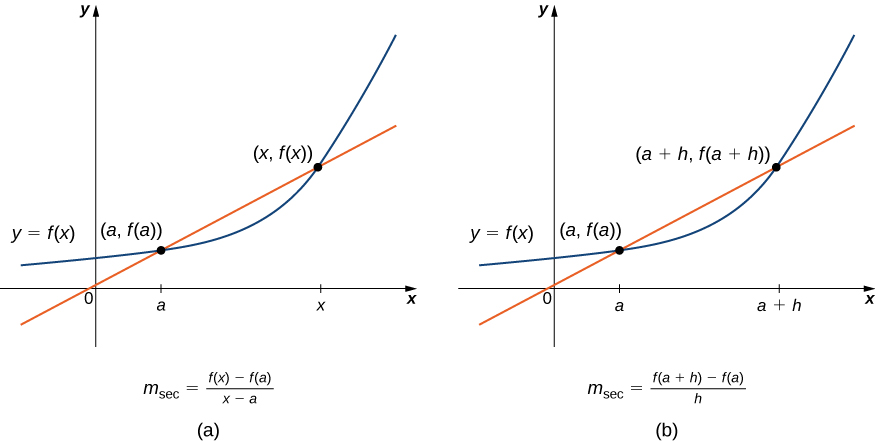
Let’s start by revisiting the notion of secant lines and tangent lines. The slope of a secant line to a function at a point [latex](a,f(a))[/latex] helps estimate the rate of change. We can find the slope of the secant by choosing a value of [latex]x[/latex] near [latex]a[/latex] and drawing a line through the points [latex](a,f(a))[/latex] and [latex](x,f(x))[/latex]. The slope of this line is given by the difference quotient:
We can also calculate the slope of a secant line to a function at a value [latex]a[/latex] by using this equation and replacing [latex]x[/latex] with [latex]a+h[/latex], where [latex]h[/latex] is a value close to [latex]0[/latex]. This gives us the slope of the secant line through the points [latex](a,f(a))[/latex] and [latex](a+h,f(a+h))[/latex]:
difference quotient
Let [latex]f[/latex] be a function defined on an interval [latex]I[/latex] containing [latex]a[/latex]. If [latex]x\ne a[/latex] is in [latex]I[/latex], then
is a difference quotient.
Also, if [latex]h\ne 0[/latex] is chosen so that [latex]a+h[/latex] is in [latex]I[/latex], then
is a difference quotient with increment [latex]h[/latex].
These two expressions for calculating the slope of a secant line are illustrated in Figure 2. Depending on the setting, we can choose either method based on ease of calculation.
In Figure 3(a), as the values of [latex]x[/latex] approach [latex]a[/latex], the slopes of the secant lines provide better estimates of the rate of change of the function at [latex]a[/latex]. The secant lines themselves approach the tangent line to the function at [latex]a[/latex], which represents the limit of the secant lines. Similarly, Figure 3(b) shows that as the values of [latex]h[/latex] get closer to [latex]0[/latex], the secant lines also approach the tangent line. The slope of the tangent line at [latex]a[/latex] is the rate of change of the function at [latex]a[/latex], as shown in Figure 3(c).
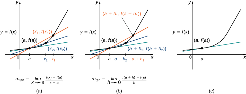
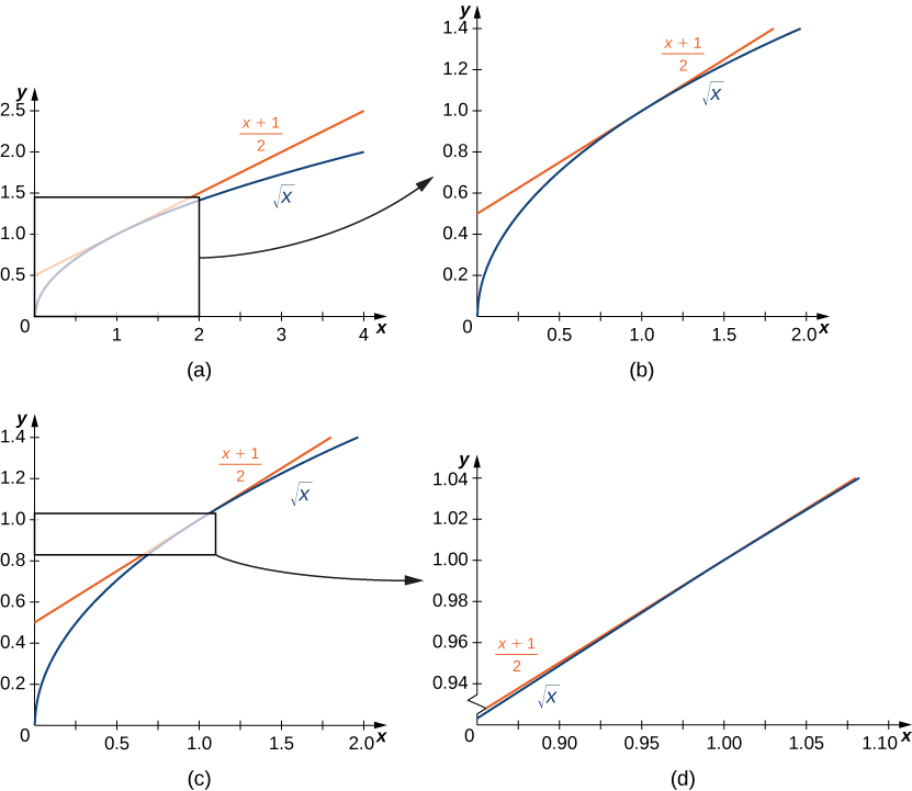
Figure 4 shows the graph of [latex]f(x)=\sqrt{x}[/latex] and its tangent line at [latex](1,1)[/latex] in a series of tighter intervals about [latex]x=1[/latex]. As the intervals narrow, the graph of the function and its tangent line appear to coincide, making the values on the tangent line a goodapproximation of the function near [latex]x =1[/latex]. In fact, the graph of [latex]f(x)[/latex] appears locally linear close to [latex]x=1[/latex].
Formally we may define the tangent line to the graph of a function as follows.
tangent line
Let [latex]f(x)[/latex] be a function defined in an open interval containing [latex]a[/latex]. The tangent line to [latex]f(x)[/latex] at [latex]a[/latex] is the line passing through the point [latex](a,f(a))[/latex] having slope
provided this limit exists.
Equivalently, we may define the tangent line to [latex]f(x)[/latex] at [latex]a[/latex] to be the line passing through the point [latex](a,f(a))[/latex] having slope
provided this limit exists.
Just as we used two expressions to define the slope of a secant line, we use two forms to define the slope of a tangent line. In this text, we use both definitions depending on the context.
Now that we have defined a tangent line to a function at a point, we can find equations of tangent lines. This requires recalling two algebraic techniques: evaluating a function with variable inputs and using point-slope form to write an equation of a line.
- Evaluating Functions: Functions can be evaluated for inputs that are variables or expressions. The process is the same as evaluating with a constant, but the simplified answer will contain a variable.
- Point-Slope Form: The point-slope form of a linear equation takes the form:
[latex]y-{y}_{1}=m\left(x-{x}_{1}\right)[/latex]
where [latex]m[/latex] is the slope, and [latex](x_1,y_1)[/latex] are the coordinates of a specific point through which the line passes.
Find the equation of the line tangent to the graph of [latex]f(x)=x^2[/latex] at [latex]x=3[/latex].
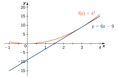
Use the second definition to find the slope of the line tangent to the graph of [latex]f(x)=x^2[/latex] at [latex]x=3[/latex].