Transformations of Functions 

Understanding how to transform the graph of a function is essential in visualizing mathematical concepts. Transformations include shifting, stretching, or reflecting the graph. Shifting moves the graph up, down, left, or right, stretching alters its width or height, and reflecting flips it over an axis.

Vertical Shift

Vertical shifts in graphs occur when each point on the graph moves up or down by the same amount. This shift is the result of adding or subtracting a constant to the function’s output value [latex]y[/latex].

For a positive constant [latex]c[/latex], adding it to a function [latex]f(x)[/latex] results in [latex]f(x)+c[/latex], raising the graph up [latex]c[/latex] units. Conversely, subtracting [latex]c[/latex] from [latex]f(x)[/latex] to get [latex]f(x)-c[/latex] lowers the graph by [latex]c[/latex] units. These shifts do not affect the shape of the graph; they simply reposition it along the [latex]y[/latex]-axis.

vertical shift

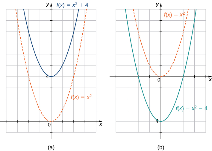
Vertical shifts do not alter the shape of a function’s graph, only its position along the [latex]y[/latex]-axis. Adding a positive constant lifts the graph upwards, while subtracting it pushes the graph downwards.

The graph of the function [latex]f(x)=x^3+4[/latex] is the graph of [latex]y=x^3[/latex] shifted up 4 units; the graph of the function [latex]f(x)=x^3-4[/latex] is the graph of [latex]y=x^3[/latex] shifted down [latex]4[/latex] units (Figure 15).

Horizontal Shift

Horizontal shifts in function graphs reflect the influence of adding or subtracting a constant from each input value [latex]x[/latex].

For a positive constant [latex]c[/latex], subtracting it from [latex]x[/latex] to form [latex]f(x-c)[/latex] shifts the graph to the right by [latex]c[/latex] units. In contrast, adding [latex]c[/latex] to [latex]x[/latex], resulting in  [latex]f(x+c)[/latex], moves the graph to the left by [latex]c[/latex] units.

horizontal shift

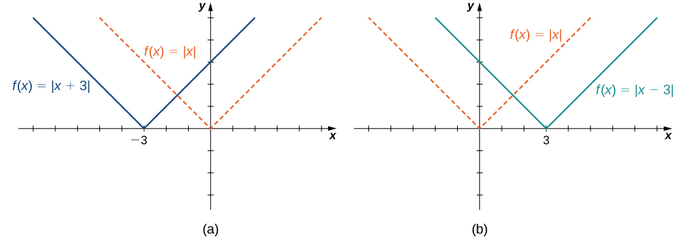
Horizontal shifts alter the position of a function’s graph along the [latex]x[/latex]-axis but do not change its shape. Subtracting a positive constant from the input moves the graph to the right, while adding it shifts the graph to the left

Why does the graph shift left when adding a constant and shift right when subtracting a constant? To answer this question, let’s look at an example.

Consider the function [latex]f(x)=|x+3|[/latex] and evaluate this function at [latex]x-3.[/latex] Since [latex]f(x-3)=|x|[/latex] and [latex]x-3 < x[/latex], the graph of [latex]f(x)=|x+3|[/latex] is the graph of [latex]y=|x|[/latex] shifted left [latex]3[/latex] units. Similarly, the graph of [latex]f(x)=|x-3|[/latex] is the graph of [latex]y=|x|[/latex] shifted right [latex]3[/latex] units (Figure 16).

Vertical Scaling (Stretched/Compressed)

A vertical scaling of a graph occurs if we multiply all outputs [latex]y[/latex] of a function by the same positive constant [latex]c[/latex].

If [latex]c>1[/latex], the graph of the function [latex]cf(x)[/latex] appears vertically stretched, as the outputs are proportionally larger than those of the original function [latex]f(x)[/latex]. If [latex]0 < c <1[/latex], then the outputs of the function [latex]cf(x)[/latex] are smaller, so the graph has been compressed, resulting in a graph that is closer to the [latex]x[/latex]-axis.

vertical scaling

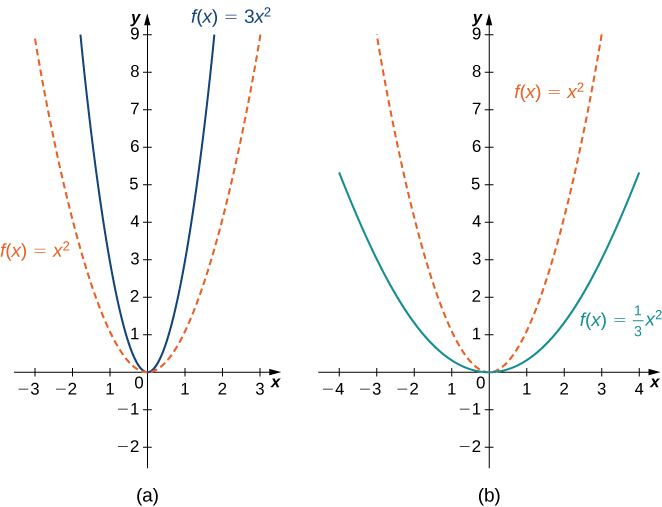
Vertical scaling changes the steepness of a function’s graph. Multiplying by a constant greater than [latex]1[/latex] stretches the graph away from the [latex]x[/latex]-axis, while multiplying by a constant between [latex]0[/latex] and [latex]1[/latex] compresses it towards the [latex]x[/latex]-axis.

The graph of the function [latex]f(x)=3x^2[/latex] is the graph of [latex]y=x^2[/latex] stretched vertically by a factor of [latex]3[/latex], whereas the graph of [latex]f(x)=\frac{x^2}{3}[/latex] is the graph of [latex]y=x^2[/latex] compressed vertically by a factor of [latex]3[/latex] (Figure 17).

Horizontal Scaling (Stretched/Compressed)

Horizontal scaling modifies the width of a function’s graph by stretching or compressing it along the [latex]x[/latex]-axis. This effect is achieved by multiplying the input, [latex]x[/latex], by a constant [latex]c[/latex].

When [latex]c>0[/latex], the function [latex]f(cx)[/latex] is the graph of [latex]f(x)[/latex] is compressed, as each input value is effectively scaled down, bringing the points closer together horizontally. If [latex]0 < c <1[/latex], the function [latex]f(cx)[/latex] is stretched, because the input values are scaled up, spreading the points further apart on the [latex]x[/latex]-axis.

horizontal scaling

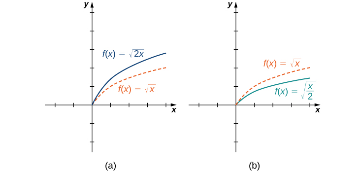
Horizontal scaling affects the horizontal spread of a function’s graph. Multiplying the input by a constant greater than [latex]1[/latex] compresses the graph, while a constant between [latex]0[/latex] and [latex]1[/latex] stretches it.

Consider the function [latex]f(x)=\sqrt{2x}[/latex] and evaluate [latex]f[/latex] at [latex]\dfrac{x}{2}.[/latex] Since [latex]f(\frac{x}{2})=\sqrt{x}[/latex], the graph of [latex]f(x)=\sqrt{2x}[/latex] is the graph of [latex]y=\sqrt{x}[/latex] compressed horizontally. The graph of [latex]y=\sqrt{\frac{x}{2}}[/latex] is a horizontal stretch of the graph of [latex]y=\sqrt{x}[/latex] (Figure 18).

Reflection

Reflections of a function’s graph across an axis create a mirror image. When we multiply the outputs of a function, [latex]f(x)[/latex], by [latex]-1[/latex] we achieve a reflection across the [latex]x[/latex]-axis, turning every point to its opposite position vertically. Similarly, multiplying the inputs by [latex]-1[/latex] before applying the function, as in [latex]f(-x)[/latex], reflects the graph across the y-axis, flipping it horizontally. 

reflections of functions

Reflecting a function’s graph across an axis is accomplished by multiplying by[latex]-1[/latex]. To mirror across the [latex]x[/latex]-axis, multiply the outputs by [latex]-1[/latex]. To reflect across the [latex]y[/latex]-axis, multiply the inputs by [latex]-1[/latex].

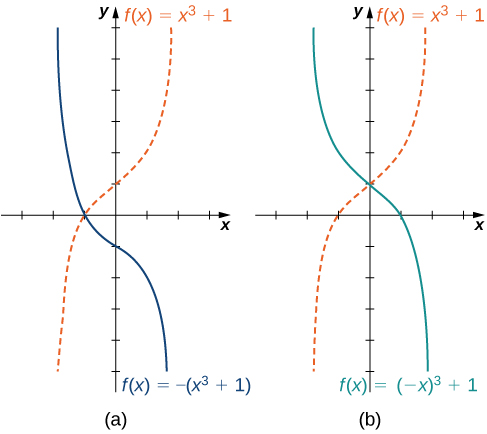
The graph of [latex]f(x)=−(x^3+1)[/latex] is the graph of [latex]y=(x^3+1)[/latex] reflected about the [latex]x[/latex]-axis. The graph of [latex]f(x)=(−x)^3+1[/latex] is the graph of [latex]y=x^3+1[/latex] reflected about the [latex]y[/latex]-axis (Figure 19).

Multiple Transformations

If the graph of a function consists of more than one transformation of another graph, it is important to transform the graph in the correct order. Given a function [latex]f(x)[/latex], the graph of the related function [latex]y=cf(a(x+b))+d[/latex] can be obtained from the graph of [latex]y=f(x)[/latex] by performing the transformations in the following order.

1. Horizontal shift of the graph of [latex]y=f(x)[/latex]. If [latex]b>0[/latex], shift left. If [latex]b<0[/latex], shift right.
2. Horizontal scaling of the graph of [latex]y=f(x+b)[/latex] by a factor of [latex]|a|[/latex]. If [latex]a<0[/latex], reflect the graph about the [latex]y[/latex]-axis.
3. Vertical scaling of the graph of [latex]y=f(a(x+b))[/latex] by a factor of [latex]|c|[/latex]. If [latex]c<0[/latex], reflect the graph about the [latex]x[/latex]-axis.
4. Vertical shift of the graph of [latex]y=cf(a(x+b))[/latex]. If [latex]d>0[/latex], shift up. If [latex]d<0[/latex], shift down.

We can summarize the different transformations and their related effects on the graph of a function in the following table.

Transformations of Functions

Transformation of [latex]f(c>0)[/latex]	Effect on the graph of[latex]f[/latex]
[latex]f(x)+c[/latex]	Vertical shift up [latex]c[/latex] units
[latex]f(x)-c[/latex]	Vertical shift down [latex]c[/latex] units
[latex]f(x+c)[/latex]	Shift left by [latex]c[/latex] units
[latex]f(x-c)[/latex]	Shift right by [latex]c[/latex] units
[latex]cf(x)[/latex]	Vertical stretch if [latex]c>1[/latex]; vertical compression if [latex]0 < c < 1[/latex]
[latex]f(cx)[/latex]	Horizontal stretch if [latex]0 < c < 1[/latex]; horizontal compression if [latex]c>1[/latex]
[latex]−f(x)[/latex]	Reflection about the [latex]x[/latex]-axis
[latex]f(−x)[/latex]	Reflection about the [latex]y[/latex]-axis

Describe how the function [latex]f(x)=−(x+1)^2-4[/latex] can be graphed using the graph of [latex]y=x^2[/latex] and a sequence of transformations.

Show Solution

To graph the function [latex]f(x)=−(x+1)^2-4[/latex] using transformations, start with the base function [latex]g(x)=x^2[/latex] and follow these steps:

1. Horizontal Shift: The term [latex](x+1)[/latex] within [latex](x+1)^2[/latex] indicates a horizontal shift of the graph of [latex]g(x)[/latex] one unit to the left. 
2. Vertical Shift: The [latex]−4[/latex] at the end of [latex](x+1)^2−4[/latex] indicates a vertical shift downward by [latex]4[/latex] units. This is a result of subtracting [latex]4[/latex] from the entire squared term.
3. Reflection: The negative sign in front of the function indicates that the graph will be a reflection of [latex]g(x)=x^2[/latex] across the [latex]x[/latex]-axis. This means that the parabola, which normally opens upwards, will now open downwards.

To graph [latex]f(x)[/latex]:

• Begin with the graph of [latex]g(x)=x^2[/latex], which is a parabola with its vertex at the origin [latex](0,0)[/latex].
• Reflecting it across the x-axis due to the negative sign, which will flip the parabola to open downwards.
• Move this graph one unit left to accommodate the [latex]+1[/latex] within the squared term, shifting the vertex to [latex](−1,0)[/latex].
• Then, shift the graph down four units for the [latex]−4[/latex], placing the vertex at [latex](−1,−4)[/latex].

The transformed graph of [latex]f(x)[/latex] will be a downward-opening parabola with its vertex at [latex](−1,−4)[/latex].

It is beneficial when working with transformations to remember the basic toolkit functions. These will be your starting points when trying to identify how the function has been transformed.

Toolkit Functions
Name	Function	Graph
Constant	[latex]f\left(x\right)=c[/latex], where [latex]c[/latex] is a constant
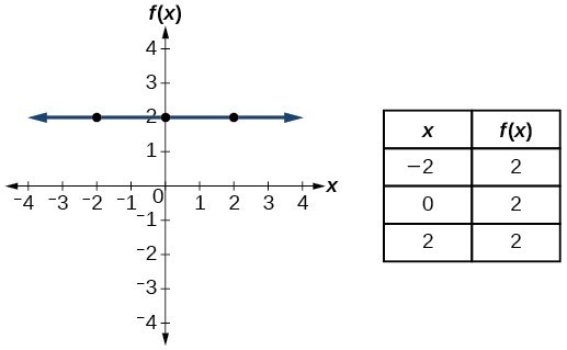Identity/Linear	[latex]f\left(x\right)=x[/latex]
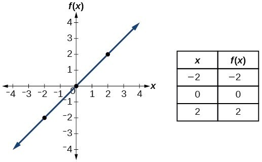Absolute value	[latex]f\left(x\right)=|x|[/latex]
Quadratic	[latex]f\left(x\right)={x}^{2}[/latex]
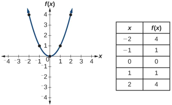Cubic	[latex]f\left(x\right)={x}^{3}[/latex]
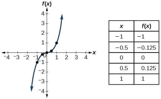Reciprocal	[latex]f\left(x\right)=\frac{1}{x}[/latex]
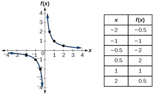Reciprocal squared	[latex]f\left(x\right)=\frac{1}{{x}^{2}}[/latex]
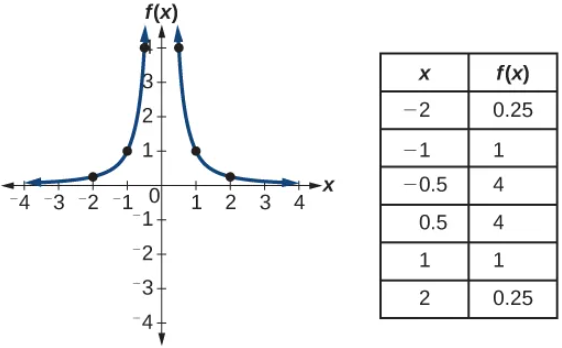Square root	[latex]f\left(x\right)=\sqrt{x}[/latex]
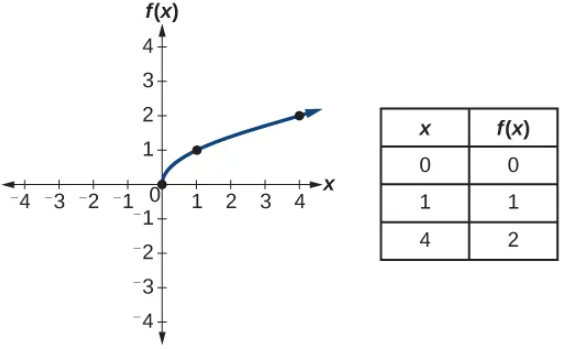Cube root	[latex]f\left(x\right)=\sqrt[3]{x}[/latex]

For each of the following functions, sketch a graph by using a sequence of transformations of a toolkit function.

1. [latex]f(x)=−|x+2|-3[/latex]
2. [latex]f(x)=3\sqrt{−x}+1[/latex]

Show Solution

1. Starting with the graph of [latex]y=|x|[/latex], shift [latex]2[/latex] units to the left, reflect about the [latex]x[/latex]-axis, and then shift down [latex]3[/latex] units.
   

   

2. Starting with the graph of [latex]y=\sqrt{x}[/latex], reflect about the [latex]y[/latex]-axis, stretch the graph vertically by a factor of [latex]3[/latex], and move up [latex]1[/latex] unit.
   

   

Watch the following video to see the worked solution to this example.

For closed captioning, open the video on its original page by clicking the Youtube logo in the lower right-hand corner of the video display. In YouTube, the video will begin at the same starting point as this clip, but will continue playing until the very end.

You can view the transcript for this video using this link (opens in new window).