Areas Between Curves: Learn It 3

Lumen Learning

Areas Between Curves: Learn It 3

Regions Defined with Respect to $y$

In the previous example, we had to evaluate two separate integrals to calculate the area of the region. However, there is another approach that requires only one integral. What if we treat the curves as functions of $y,$ instead of as functions of $x?$

Review the last example.

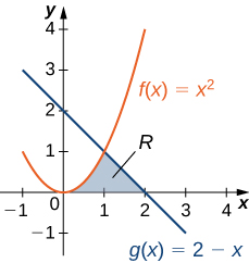
Consider the region depicted in the following figure. Find the area of $R.$

This figure is has two graphs in the first quadrant. They are the functions f(x) = squareroot of x and g(x)= 3/2 – x/2. In between these graphs is a shaded region, bounded to the left by f(x) and to the right by g(x). All of which is above the x-axis. The shaded area is between x=0 and x=3. — Figure 7.

Note that the left graph, shown in red, is represented by the function $y=f(x)={x}^{2}.$ We could just as easily solve this for $x$ and represent the curve by the function $x=v(y)=\sqrt{y}.$ However, based on the graph, it is clear we are interested in the positive square root.

Similarly, the right graph is represented by the function $y=g(x)=2-x,$ but could just as easily be represented by the function $x=u(y)=2-y.$

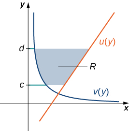
When the graphs are represented as functions of $y,$ we see the region is bounded on the left by the graph of one function and on the right by the graph of the other function. Therefore, if we integrate with respect to $y,$ we need to evaluate only one integral.

Let’s develop a formula for this type of integration.

Let $u(y)$ and $v(y)$ be continuous functions over an interval $\left[c,d\right]$ such that $u(y)\ge v(y)$ for all $y\in \left[c,d\right].$ We want to find the area between the graphs of the functions, as shown in the following figure.

This figure is has two graphs in the first quadrant. They are the functions v(y) and u(y). In between these graphs is a shaded region, bounded to the left by v(y) and to the right by u(y). The region is labeled R. The shaded area is between the horizontal boundaries of y=c and y=d. — Figure 8. We can find the area between the graphs of two functions, $u(y)$ and $v(y).$

This time, we are going to partition the interval on the $y\text{-axis}$ and use horizontal rectangles to approximate the area between the functions. So, for $i=0,1,2\text{,…},n,$ let $Q=\left\{{y}_{i}\right\}$ be a regular partition of $\left[c,d\right].$ Then, for $i=1,2\text{,…},n,$ choose a point ${y}_{i}^{*}\in \left[{y}_{i-1},{y}_{i}\right],$ then over each interval $\left[{y}_{i-1},{y}_{i}\right]$ construct a rectangle that extends horizontally from $v({y}_{i}^{*})$ to $u({y}_{i}^{*}).$

This figure is has three graphs. The first figure has two curves. They are the functions v(y*) and u(y*). In between these curves is a horizontal rectangle. The second figure labeled “(a)”, is a shaded region, bounded to the left by v(y) and to the right by u(y). The shaded area is between the horizontal boundaries of y=c and y=d. This shaded area is broken into rectangles between the curves. The third figure, labeled “(b)”, is the two curves v(y*) and u(y*). In between the curves is a horizontal rectangle with width delta y. — Figure 9. (a) Approximating the area between the graphs of two functions, $u(y)$ and $v(y),$ with rectangles. (b) The area of a typical rectangle.

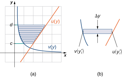
The height of each individual rectangle is $\text{Δ}y$ and the width of each rectangle is $u({y}_{i}^{*})-v({y}_{i}^{*}).$ Adding the areas of all the rectangles, we see that the area between the curves is approximated by:

A \approx \underset{i = 1}{∑^{n}} [u (y_{i}^{*}) - v (y_{i}^{*})] Δ y .

$A\approx \underset{i=1}{\overset{n}{\text{∑}}}\left[u({y}_{i}^{*})-v({y}_{i}^{*})\right]\text{Δ}y.$

This is a Riemann sum, so we take the limit as $n\to \infty ,$ and we get:

A = lim_{n \to \infty} \underset{i = 1}{∑^{n}} [u (y_{i}^{*}) - v (y_{i}^{*})] Δ y = \int_{c}^{d} [u (y) - v (y)] d y .

$A=\underset{n\to \infty }{\text{lim}}\underset{i=1}{\overset{n}{\text{∑}}}\left[u({y}_{i}^{*})-v({y}_{i}^{*})\right]\text{Δ}y={\displaystyle\int }_{c}^{d}\left[u(y)-v(y)\right]dy.$

These findings are summarized in the following theorem.

finding the area between two curves, integrating along the $y$ -axis

Let $u(y)$ and $v(y)$ be continuous functions such that $u(y)\ge v(y)$ for all $y\in \left[c,d\right].$

Let $R$ denote the region bounded on the right by the graph of $u(y),$ on the left by the graph of $v(y),$ and above and below by the lines $y=d$ and $y=c,$ respectively.

Then, the area of $R$ is given by:

A = \int_{c}^{d} [u (y) - v (y)] d y .

$A={\displaystyle\int }_{c}^{d}\left[u(y)-v(y)\right]dy.$

Back to our previous example, let’s integrate with respect to $y$ . Let $R$ be the region depicted in the following figure. Find the area of $R$ by integrating with respect to $y.$

$\frac{5}{3}$ units²

Watch the following video to see the worked solution to this example.

For closed captioning, open the video on its original page by clicking the Youtube logo in the lower right-hand corner of the video display. In YouTube, the video will begin at the same starting point as this clip, but will continue playing until the very end.

You can view the transcript for this segmented clip of “2.1 Area Between Curves” here (opens in new window).

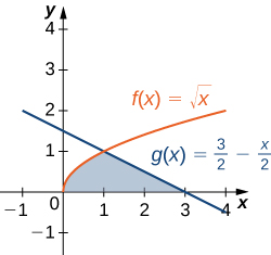
Let $R$ be the region depicted in the figure below. Find the area of $R$ by integrating with respect to $y.$

This figure is has two graphs in the first quadrant. They are the functions f(x) = x^2 and g(x)= 2-x. In between these graphs is a shaded region, bounded to the left by f(x) and to the right by g(x). All of which is above the x-axis. The region is labeled R. The shaded area is between x=0 and x=2. — Figure 10. The area of region $R$ can be calculated using one integral only when the curves are treated as functions of $y.$

We must first express the graphs as functions of $y.$ As we saw at the beginning of this section, the curve on the left can be represented by the function $x=v(y)=\sqrt{y},$ and the curve on the right can be represented by the function $x=u(y)=2-y.$

Now we have to determine the limits of integration.

The region is bounded below by the $x$ -axis, so the lower limit of integration is $y=0.$ The upper limit of integration is determined by the point where the two graphs intersect, which is the point $(1,1),$ so the upper limit of integration is $y=1.$

Thus, we have $\left[c,d\right]=\left[0,1\right].$

Calculating the area of the region, we get:

\begin{array}{cc} A & = \int_{c}^{d} [u (y) - v (y)] d y \\ = \int_{0}^{1} [(2 - y) - \sqrt{y}] d y = {[2 y - \frac{y^{2}}{2} - \frac{2}{3} y^{3 / 2}] |}_{0}^{1} \\ = \frac{5}{6} . \end{array}

$\begin{array}{cc}\hfill A& ={\displaystyle\int }_{c}^{d}\left[u(y)-v(y)\right]dy\hfill \\ & ={\displaystyle\int }_{0}^{1}\left[(2-y)-\sqrt{y}\right]dy={\left[2y-\frac{{y}^{2}}{2}-\frac{2}{3}{y}^{3\text{/}2}\right]|}_{0}^{1}\hfill \\ & =\frac{5}{6}.\hfill \end{array}$

The area of the region is $\frac{5}{6}$ units².

Areas Between Curves: Learn It 3

Regions Defined with Respect to yyy

finding the area between two curves, integrating along the yyy-axis

Regions Defined with Respect to $y$

finding the area between two curves, integrating along the $y$ -axis