- Calculate the length of a curve described by y=f(x) from one point to another
- Find the length of a curve defined by x=g(y) from one point to another
- Calculate the total surface area of a solid formed by rotating a curve around an axis
Arc Lengths of Curves
In this section, we use definite integrals to find the arc length of a curve. We can think of arc length as the distance you would travel if you were walking along the path of the curve.
Many real-world applications involve arc length. If a rocket is launched along a parabolic path, we might want to know how far the rocket travels. Or, if a curve on a map represents a road, we might want to know how far we have to drive to reach our destination.
Arc Length of the Curve [latex]y[/latex] = [latex]f[/latex]([latex]x[/latex])
In previous applications of integration, we required the function [latex]f(x)[/latex] to be integrable, or at most continuous. However, for calculating arc length we have a more stringent requirement for [latex]f(x).[/latex] Here, we require [latex]f(x)[/latex] to be differentiable, and furthermore we require its derivative, [latex]{f}^{\prime }(x),[/latex] to be continuous. Functions like this, which have continuous derivatives, are called smooth.
Let [latex]f(x)[/latex] be a smooth function defined over [latex]\left[a,b\right].[/latex] We want to calculate the length of the curve from the point [latex](a,f(a))[/latex] to the point [latex](b,f(b)).[/latex]
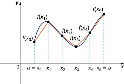
We start by using line segments to approximate the length of the curve.
For [latex]i=0,1,2\text{,…},n,[/latex] let [latex]P=\left\{{x}_{i}\right\}[/latex] be a regular partition of [latex]\left[a,b\right].[/latex]
Then, for [latex]i=1,2\text{,…},n,[/latex] construct a line segment from the point [latex]({x}_{i-1},f({x}_{i-1}))[/latex] to the point [latex]({x}_{i},f({x}_{i})).[/latex] Although it might seem logical to use either horizontal or vertical line segments, we want our line segments to approximate the curve as closely as possible. The figure below depicts this construct for [latex]n=5.[/latex]
To help us find the length of each line segment, we look at the change in vertical distance as well as the change in horizontal distance over each interval.
Because we have used a regular partition, the change in horizontal distance over each interval is given by [latex]\text{Δ}x.[/latex] The change in vertical distance varies from interval to interval, though, so we use [latex]\text{Δ}{y}_{i}=f({x}_{i})-f({x}_{i-1})[/latex] to represent the change in vertical distance over the interval [latex]\left[{x}_{i-1},{x}_{i}\right],[/latex] as shown below Note that some (or all) [latex]\text{Δ}{y}_{i}[/latex] may be negative.
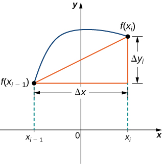
By the Pythagorean theorem, the length of the line segment is:
[latex]\sqrt{{(\text{Δ}x)}^{2}+{(\text{Δ}{y}_{i})}^{2}}.[/latex]
We can also write this as:
[latex]\text{Δ}x\sqrt{1+{((\text{Δ}{y}_{i})\text{/}(\text{Δ}x))}^{2}}.[/latex]
Now, by the Mean Value Theorem, there is a point [latex]{x}_{i}^{*}\in \left[{x}_{i-1},{x}_{i}\right][/latex] such that [latex]{f}^{\prime }({x}_{i}^{*})=(\text{Δ}{y}_{i})\text{/}(\text{Δ}x).[/latex]
Then the length of the line segment is given by:
[latex]\text{Δ}x\sqrt{1+{\left[{f}^{\prime }({x}_{i}^{*})\right]}^{2}}.[/latex]
Adding up the lengths of all the line segments, we get:
This is a Riemann sum. Taking the limit as [latex]n\to \infty ,[/latex] we have:
We summarize these findings in the following theorem.
arc length for [latex]y[/latex] = [latex]f[/latex]([latex]x[/latex])
Let [latex]f(x)[/latex] be a smooth function over the interval [latex]\left[a,b\right].[/latex] Then the arc length of the portion of the graph of [latex]f(x)[/latex] from the point [latex](a,f(a))[/latex] to the point [latex](b,f(b))[/latex] is given by:
Note that we are integrating an expression involving [latex]{f}^{\prime }(x),[/latex] so we need to be sure [latex]{f}^{\prime }(x)[/latex] is integrable. This is why we require [latex]f(x)[/latex] to be smooth. The following example shows how to apply the theorem.
Let [latex]f(x)=2{x}^{3\text{/}2}.[/latex] Calculate the arc length of the graph of [latex]f(x)[/latex] over the interval [latex]\left[0,1\right].[/latex] Round the answer to three decimal places.
Although it is nice to have a formula for calculating arc length, this particular theorem can generate expressions that are difficult to integrate. In some cases, we may have to use a computer or calculator to approximate the value of the integral.
Let [latex]f(x)={x}^{2}.[/latex] Calculate the arc length of the graph of [latex]f(x)[/latex] over the interval [latex]\left[1,3\right].[/latex]