• Understand that while all differentiable functions can be derived in a straightforward formula, not all functions can be integrated into a simple antiderivative
• Calculate bounds for the area calculations under curves when direct integration methods aren’t applicable
• Explain how estimating the bounds of an integral affects the accuracy of the approximation

Approximating Integrals

At this point on our calculus journey, we have developed the tools to find the derivative function of any differentiable function. Take, for example, the following function.

[latex]f(x)=\left[\ln\left(\tan^2\left(\frac{1}{x^{2}+3\sqrt{x}}\right)\right)\cos^{-1}\left(\frac{3x^{2}+5x-1}{22x+1}\right)+10x^{3^{x^{2}}}\right]^{e^{\sin(x^{3.2})}}[/latex]

Finding the derivative of this function would take multiple pages using the Chain Rule, Quotient Rule, Product Rule, Sum Rule, and derivative formulas. By cutting some corners and letting Wolfram|Alpha find the derivative function for us, we see that it is:

Don’t worry—we won’t be asked to do anything quite that crazy by hand. But the point is that for any differentiable function we are given, we can apply the tools in our calculus toolbelt to find the closed-form expression of its derivative function.

However, integration is not always straightforward. There are many functions which are integrable but have no antiderivative in terms of standard elementary functions we’ve seen so far.

Consider:

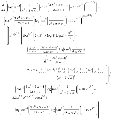
[latex]g(x)=\frac{1}{\sqrt{2\pi}}e^{-\frac{1}{2}x^{2}}[/latex]

If we were asked to compute the definite integral [latex]\displaystyle\int _{0}^{1} g(x)dx[/latex], the graphical area of which is shown in the figure below, could we use the Fundamental Theorem of Calculus, Part 2?

Try this on your own for a moment. Can you find an antiderivative of [latex]g(x)[/latex] in terms of elementary functions?

If your conclusion is “no,” then you are correct. While the function looks simple, it does not have an antiderivative in terms of elementary functions.

In Calculus II, we will learn additional techniques to find antiderivatives and indefinite integrals, such as integration by parts and partial fraction decomposition. However, even these methods cannot help us with the function [latex]g(x)[/latex].

Finding an antiderivative of [latex]g(x)[/latex] requires introducing special functions that are themselves defined in terms of integrals. This makes the process too complicated to apply the Fundamental Theorem of Calculus, Part 2, directly. (If you’re curious, you can look up the error function [latex]\text{erf}(x)[/latex].

So, what can we do to find [latex]\displaystyle\int _{0}^{1} g(x)dx[/latex] if we cannot find an antiderivative of [latex]g(x)[/latex] in terms of elementary functions? We approximate the definite integral!

Remember, earlier in this module, we learned about using Riemann Sums to approximate the area under a curve. This method may not give us an exact answer but can get us very close when we’ve exhausted other tools. There are also tricks in mathematics that make approximations extremely useful.

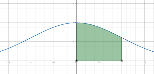
Let’s use a left-endpoint Riemann Sum to approximate [latex]\displaystyle\int _{0}^{1} g(x)dx[/latex] where [latex]g(x)[/latex] is defined as above. If we split the interval [latex][0,1][/latex] into [latex]n[/latex] subintervals of length [latex]\frac{1}{n}[/latex], then the left-endpoint Riemann sum is:

[latex]L_{n}={\displaystyle\sum _{i=1}^{n}} g\left(\frac{i-1}{n}\right)\cdot\frac{1}{n}[/latex].

If we choose [latex]n=10[/latex], then our approximation would be:

[latex]{\displaystyle\int _{0}^{1}} \frac{1}{\sqrt{2\pi}}e^{-\frac{1}{2}x^{2}}dx\approx L_{10}={\displaystyle\sum_{i=1}^{10}}\left[\frac{1}{\sqrt{2\pi}}e^{-\frac{1}{2}(i-1/10)^{2}}\cdot\frac{1}{10}\right]\approx0.349[/latex].

Graphically, this left-endpoint sum with [latex]10[/latex] subintervals looks as follows.

If we tell someone, “We have an approximation for [latex]\displaystyle\int _{0}^{1} g(x)dx[/latex], and it is [latex]0.349[/latex]!” they might ask, “That’s great, but how close is your approximation to the true value? How large could your error be?” This is where the concept of bounds comes in handy.

Instead of just giving a single approximation, we can provide upper and lower bounds for the true value. This gives more information because it tells us an interval within which the true value lies. If we choose a value from this interval as our approximation, we can also determine the maximum possible error.

To find these bounds, we use the concepts of upper sums and lower sums.

An upper sum uses the maximum function value on each subinterval, giving a weak over-approximation of the true area. A lower sum uses the minimum function value on each subinterval, giving a weak under-approximation of the true area.

Therefore, we can state:

[latex]\text{Lower Sum}\le\text{True Value}\le\text{Upper Sum}[/latex].

In our example, [latex]g(x)=\frac{1}{\sqrt{2\pi}} e^{-\frac{1}{2}x^2}[/latex] is decreasing over the interval [latex][0,1][/latex]. Therefore, left endpoints of subintervals give maximum function values, making left-endpoint Riemann sums upper sums. Right endpoints give minimum function values, making right-endpoint Riemann sums lower sums.

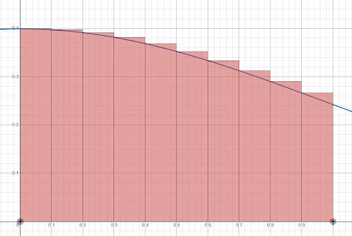
A right-endpoint Riemann Sum to approximate [latex]\displaystyle\int _{0}^{1} g(x)dx[/latex] with [latex]n[/latex] subintervals is:

[latex]R_{n}={\displaystyle\sum _{i=1}^{n}} g\left(\frac{i}{n}\right)\cdot\frac{1}{n}[/latex]

With [latex]n=10[/latex], our right-endpoint approximation is:

[latex]{\displaystyle\int _{0}^{1}} \frac{1}{\sqrt{2\pi}}e^{-\frac{1}{2}x^{2}}dx\approx R_{10}={\displaystyle\sum_{i=1}^{10}}\left[\frac{1}{\sqrt{2\pi}}e^{-\frac{1}{2}(i/10)^{2}}\cdot\frac{1}{10}\right]\approx0.333[/latex].

Graphically, this right-endpoint sum with [latex]10[/latex] subintervals looks as follows.

Now we have an upper sum [latex]L_{10}[/latex] and a lower sum [latex]R_{10}[/latex], meaning we can state:

[latex]R_{10}\le\displaystyle\int _{0}^{1} g(x)dx\le L_{10}[/latex].

Therefore,

[latex]0.333\le{\displaystyle\int _{0}^{1}} \frac{1}{\sqrt{2\pi}}e^{-\frac{1}{2}x^{2}}dx\le 0.349[/latex].

Another way to express this is that the true value of [latex]{\displaystyle\int _{0}^{1}} \frac{1}{\sqrt{2\pi}}e^{-\frac{1}{2}x^{2}}dx[/latex] must lie in the interval [latex][0.333, 0.349][/latex]. If we choose a value from that interval for our approximation, what is the maximum possible error from the true value?

Suppose we choose the midpoint of the interval [latex][0.333,0.349][/latex], which is:

[latex]\text{midpoint }=\frac{0.333+0.349}{2}=0.341[/latex].

Since the true value lies within [latex][0.333,0.349][/latex], the maximum distance our approximation could be from [latex]{\displaystyle\int _{0}^{1}} \frac{1}{\sqrt{2\pi}}e^{-\frac{1}{2}x^{2}}dx[/latex] is the distance from the midpoint to the endpoints of the interval. Let [latex]\varepsilon (x)[/latex] be the maximum error that could be associated with the approximation [latex]x[/latex]. Then,

[latex]\varepsilon(0.341)=0.349-0.341=0.341-0.333=0.008[/latex].

In words, our approximation [latex]0.341[/latex] could be at most [latex]0.008[/latex] away from the true value of from the true value of [latex]{\displaystyle\int _{0}^{1}} \frac{1}{\sqrt{2\pi}}e^{-\frac{1}{2}x^{2}}dx[/latex].

There is no specific reason we chose [latex]n=10[/latex] for the number of subintervals. As we choose larger and larger [latex]n[/latex], the interval for our approximation would become smaller, as would the maximum error. Computers can perform these calculations efficiently for very large [latex]n[/latex], often necessary when computing a definite integral for a function with no antiderivative in terms of elementary functions.

Consider the function [latex]f(x)=\sqrt{1-x^{4}}[/latex]. Can you find [latex]\displaystyle\int _{-1}^{0} f(x)dx[/latex] using the Fundamental Theorem of Calculus, Part 2? If not, provide an upper bound and a lower bound for the true value of the definite integral. If you were to choose a single value from that interval to use as an approximation, what is the maximum error that could be associated with that approximation?

Show Answer

Finding an antiderivative for [latex]f(x) = \sqrt{1 - x^4}[/latex] in terms of elementary functions is not straightforward. Thus, we cannot directly apply the Fundamental Theorem of Calculus, Part 2.

Since we cannot find an antiderivative, we will approximate the definite integral using Riemann sums and provide an upper and lower bound for the true value of the integral.

We are approximating the integral over the interval [latex][-1, 0][/latex]. Let’s split this interval into [latex]n[/latex] equal subintervals.

For simplicity, let [latex]n = 10[/latex].

For the left-endpoint sum: 

[latex]L_{n} = \sum_{i=1}^{n} f\left(a + (i-1)\Delta x\right) \Delta x[/latex]

For the right-endpoint sum:

[latex]R_{n} = \sum_{i=1}^{n} f\left(a + i\Delta x\right) \Delta x[/latex]

Where [latex]\Delta x = \frac{b-a}{n} = \frac{0 - (-1)}{10} = 0.1[/latex].

So the left-endpoint Riemann sum is:

[latex]L_{10} = \sum_{i=1}^{10} \sqrt{1 - \left(-1 + (i-1) \cdot 0.1\right)^4} \cdot 0.1[/latex]

And the right-endpoint Riemann sum is:

[latex]R_{10} = \sum_{i=1}^{10} \sqrt{1 - \left(-1 + i \cdot 0.1\right)^4} \cdot 0.1[/latex]

Calculating these sums:

[latex]L_{10} \approx 0.360[/latex] [latex]R_{10} \approx 0.332[/latex]

Establishing the bounds:

[latex]R_{10} \leq \int_{-1}^{0} \sqrt{1 - x^4} , dx \leq L_{10}[/latex]

So,

[latex]0.332 \leq \int_{-1}^{0} \sqrt{1 - x^4} , dx \leq 0.360[/latex]

Let’s choose the midpoint of the interval [latex][0.332, 0.360][/latex]:

[latex]\text{midpoint} = \frac{0.332 + 0.360}{2} = 0.346[/latex]

The maximum possible error would be the distance from the midpoint to either endpoint:

[latex]\varepsilon(0.346) = 0.360 - 0.346 = 0.346 - 0.332 = 0.014[/latex]

Thus, the maximum error associated with the approximation [latex]0.346[/latex] is [latex]0.014[/latex].