Approximating Area Cont.
Right-Endpoint Approximation
The second method for approximating area under a curve is the right-endpoint approximation. It is almost the same as the left-endpoint approximation, but now the heights of the rectangles are determined by the function values at the right of each subinterval.
Right-Endpoint Approximation
In the right-endpoint approximation, we estimate the area under a curve by constructing rectangles whose heights are determined by the function values at the right endpoints of subintervals.
The approximation of the area [latex]A[/latex] using [latex]n[/latex] subintervals is given by the formula:
where [latex]\Delta x =\frac{b-a}{n}[/latex] is the width of each subinterval, and [latex]x_{i}[/latex] are the right endpoints of the subintervals.

Since we have already seen how to solve using left-endpoint approximation, the right-endpoint approximation follows a similar process. The key difference is that the heights of the rectangles are determined by the function values at the right endpoints of the subintervals, rather than the left endpoints. This means:
- Left-Endpoint Approximation: Uses [latex]f(x_{i -1})[/latex] for each subinterval.
- Right-Endpoint Approximation: Uses [latex]f(x_i)[/latex] for each subinterval.
By adjusting the endpoint used, we slightly alter the position and height of the rectangles, which can affect the accuracy of the approximation depending on the behavior of the function.
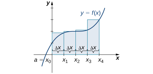
The graphs in Figure 4 represent the curve [latex]f(x)=\frac{x^2}{2}[/latex].
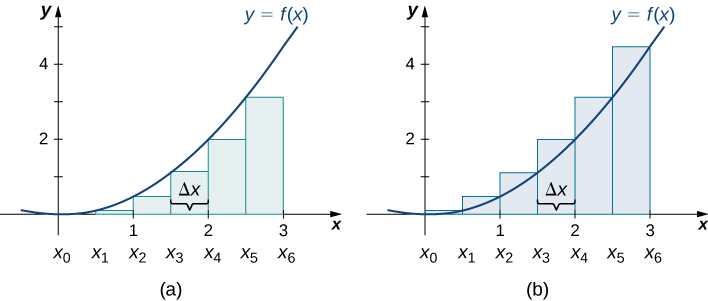
In graph (a) we divide the region represented by the interval [latex][0,3][/latex] into six subintervals, each of width [latex]0.5[/latex]. Thus, [latex]\Delta x=0.5[/latex].
We then form six rectangles by drawing vertical lines perpendicular to [latex]x_{i-1}[/latex], the left endpoint of each subinterval.
We determine the height of each rectangle by calculating [latex]f(x_{i-1})[/latex] for [latex]i=1,2,3,4,5,6[/latex].
The intervals are [latex][0,0.5], \, [0.5,1], \, [1,1.5], \, [1.5,2], \, [2,2.5], \, [2.5,3][/latex].
We find the area of each rectangle by multiplying the height by the width.
Then, the sum of the rectangular areas approximates the area between [latex]f(x)[/latex] and the [latex]x[/latex]-axis.
When the left endpoints are used to calculate height, we have a left-endpoint approximation. Thus,
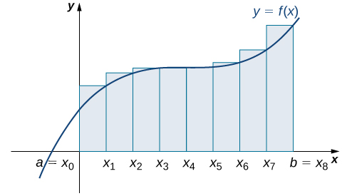
In Figure 4(b), we draw vertical lines perpendicular to [latex]x_i[/latex] such that [latex]x_i[/latex] is the right endpoint of each subinterval, and calculate [latex]f(x_i)[/latex] for [latex]i=1,2,3,4,5,6[/latex].
We multiply each [latex]f(x_i)[/latex] by [latex]\Delta x[/latex] to find the rectangular areas, and then add them. This is a right-endpoint approximation of the area under [latex]f(x)[/latex]. Thus,
Use both left-endpoint and right-endpoint approximations to approximate the area under the curve of [latex]f(x)=x^2[/latex] on the interval [latex][0,2][/latex]; use [latex]n=4[/latex].
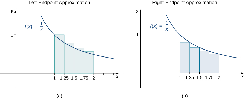
Sketch left-endpoint and right-endpoint approximations for [latex]f(x)=\frac{1}{x}[/latex] on [latex][1,2][/latex]; use [latex]n=4[/latex]. Approximate the area using both methods.
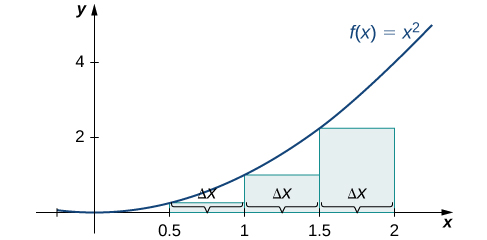
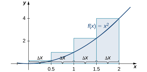
Looking at Figure 4 and the graphs in the previous example, we can see that when we use a small number of intervals, neither the left-endpoint approximation nor the right-endpoint approximation is a particularly accurate estimate of the area under the curve.
However, it seems logical that if we increase the number of points in our partition, our estimate of [latex]A[/latex] will improve. We will have more rectangles, but each rectangle will be thinner, so we will be able to fit the rectangles to the curve more precisely.
We can demonstrate the improved approximation obtained through smaller intervals with an example.
Let’s explore the idea of increasing [latex]n[/latex], first in a left-endpoint approximation with four rectangles, then eight rectangles, and finally [latex]32[/latex] rectangles. Then, let’s do the same thing in a right-endpoint approximation, using the same sets of intervals, of the same curved region.
Figure 8 shows the area of the region under the curve [latex]f(x)=(x-1)^3+4[/latex] on the interval [latex][0,2][/latex] using a left-endpoint approximation where [latex]n=4[/latex].
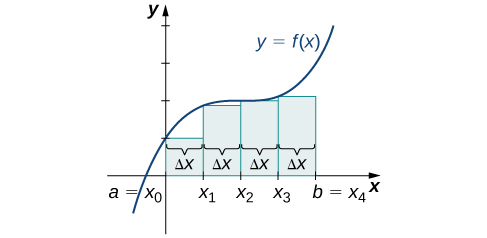
The width of each rectangle is
The area is approximated by the summed areas of the rectangles, or
Figure 9 shows the same curve divided into eight subintervals.
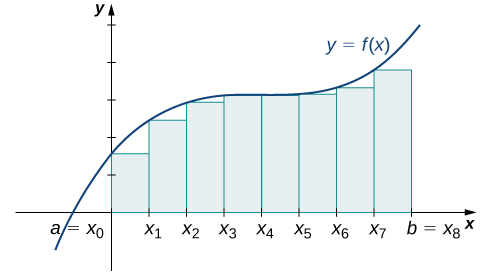
Comparing the graph with four rectangles in Figure 8 with this graph with eight rectangles, we can see there appears to be less white space under the curve when [latex]n=8[/latex]. This white space is area under the curve we are unable to include using our approximation.
The area of the rectangles is
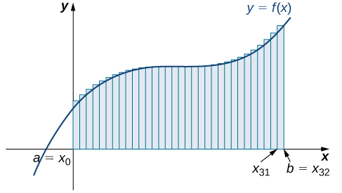
The graph in Figure 10 shows the same function with 32 rectangles inscribed under the curve.
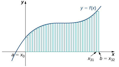
There appears to be little white space left. The area occupied by the rectangles is
We can carry out a similar process for the right-endpoint approximation method. A right-endpoint approximation of the same curve, using four rectangles (Figure 11), yields an area
Dividing the region over the interval [latex][0,2][/latex] into eight rectangles results in [latex]\Delta x=\frac{2-0}{8}=0.25[/latex]. The graph is shown in Figure 12. The area is
Last, the right-endpoint approximation with [latex]n=32[/latex] is close to the actual area (Figure 13). The area is approximately
Based on these figures and calculations, it appears we are on the right track; the rectangles appear to approximate the area under the curve better as [latex]n[/latex] gets larger.
Furthermore, as [latex]n[/latex] increases, both the left-endpoint and right-endpoint approximations appear to approach an area of [latex]8[/latex] square units.
The table below shows a numerical comparison of the left- and right-endpoint methods.
| Values of [latex]n[/latex] | Approximate Area [latex]L_n[/latex] | Approximate Area [latex]R_n[/latex] |
|---|---|---|
| [latex]n=4[/latex] | [latex]7.5[/latex] | [latex]8.5[/latex] |
| [latex]n=8[/latex] | [latex]7.75[/latex] | [latex]8.25[/latex] |
| [latex]n=32[/latex] | [latex]7.94[/latex] | [latex]8.06[/latex] |
The idea that the approximations of the area under the curve get better and better as [latex]n[/latex] gets larger and larger is very important, and we now explore this idea in more detail.