- Estimate the area under a curve by adding up the areas of rectangles
- Estimate the area under a curve using Riemann sums
Approximating Area
Archimedes used a process known as the method of exhaustion to calculate the area of various shapes. This involved using smaller and smaller shapes to approximate the area more accurately. We can use a similar method to approximate the area under a curve, [latex]f(x)[/latex], between [latex]a[/latex] and b. By dividing the area into smaller rectangles, we get closer approximations.
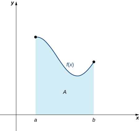
Let [latex]f(x)[/latex] be a continuous, nonnegative function defined on the closed interval [latex][a,b][/latex]. Our goal is to approximate the area [latex]A[/latex] bounded by [latex]f(x)[/latex] above, the [latex]x[/latex]-axis below, the line [latex]x=a[/latex] on the left, and the line [latex]x=b[/latex] on the right (Figure 1).
To approximate the area under this curve, we use a geometric approach. By dividing the region into many small shapes with known area formulas, we can sum these areas to estimate the true area reasonably well.
We begin by dividing the interval [latex][a,b][/latex] into [latex]n[/latex] subintervals of equal width, [latex]\frac{b-a}{n}[/latex]. We select equally spaced points [latex]x_0,x_1,x_2,\cdots,x_n[/latex] with [latex]x_0=a, \, x_n=b[/latex], and
for [latex]i=1,2,3,\cdots,n[/latex].
The width of each subinterval is denoted as [latex]\Delta x[/latex], so [latex]\Delta x=\dfrac{b-a}{n}[/latex] and the points are defined by
for [latex]i=1,2,3,\cdots,n[/latex].
This method of dividing an interval [latex][a,b][/latex] into subintervals using equally spaced points is commonly used to approximate the area under a curve. Let’s define some relevant terminology to make this process clearer.
partition
A set of points [latex]P=\{x_i\}[/latex] for [latex]i=0,1,2,\cdots,n[/latex] with [latex]a=x_0 < x_1 < x_2 < \cdots < x_n=b[/latex], which divides the interval [latex][a,b][/latex] into subintervals of the form [latex][x_0,x_1], \, [x_1,x_2],\cdots,[x_{n-1},x_n][/latex] is called a partition of [latex][a,b][/latex]. If the subintervals all have the same width, the set of points forms a regular partition of the interval [latex][a,b][/latex].
We can use this regular partition as the basis of a method for estimating the area under the curve. We next examine two methods: the left-endpoint approximation and the right-endpoint approximation.
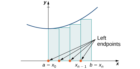
Left-Endpoint Approximation
On each subinterval [latex][x_{i-1},x_i][/latex] (for [latex]i=1,2,3,\cdots,n[/latex]), construct a rectangle with width [latex]\Delta x[/latex] and height equal to [latex]f(x_{i-1})[/latex], which is the function value at the left endpoint of the subinterval. Then the area of this rectangle is [latex]f(x_{i-1})\Delta x[/latex].
Adding the areas of all these rectangles, we get an approximate value for [latex]A[/latex]. We use the notation [latex]L_n[/latex] to denote that this is a left-endpoint approximation of [latex]A[/latex] using [latex]n[/latex] subintervals.
left-endpoint approximation
where [latex]\Delta x =\frac{b-a}{n}[/latex] is the width of each subinterval, and [latex]x_{i-1}[/latex] are the left endpoints of the subintervals.
How to: Perform Left-Endpoint Approximation
- Identify the Interval and Function: Determine the interval [latex][a,b][/latex] and the function [latex]f(x)[/latex] you are working with.
- Divide the Interval: Divide [latex][a,b][/latex] into [latex]n[/latex] subintervals of equal width [latex]\Delta x =\frac{b-a}{n}[/latex].
- Determine Left Endpoints: Identify the left endpoints of each subinterval: [latex]x_0,x_1,x_2,\cdots,x_{n-1}[/latex]
- Evaluate the Function: Calculate the function values at each left endpoint: [latex]f(x_0), f(x_1), f(x_2), \cdots, f(x_{n-1})[/latex].
- Calculate Rectangle Areas: Multiply each function value by the width [latex]Δx[/latex] to get the area of each rectangle.
- Sum the Areas: Add up all the rectangle areas to get the approximate area under the curve
[latex]A \approx \displaystyle\sum_{i=1}^{n} f(x_{i-1})\Delta x[/latex]