The Tangent Problem and Differential Calculus Cont.
The Secant Line
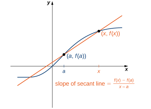
We can approximate the rate of change of a function [latex]f(x)[/latex] at a point [latex](a,f(a))[/latex] on its graph by taking another point [latex](x,f(x))[/latex] on the graph of [latex]f(x)[/latex], drawing a line through the two points, and calculating the slope of the resulting line. Such a line is called a secant line.
secant line
The secant to the function [latex]f(x)[/latex] through the points [latex](a,f(a))[/latex] and [latex](x,f(x))[/latex] is the line passing through these points. Its slope is given by
The figure below shows a secant line to a function [latex]f(x)[/latex] at a point [latex](a,f(a))[/latex].
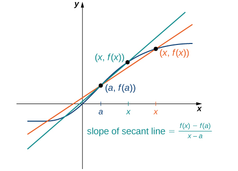
The accuracy of approximating the rate of change of the function with a secant line depends on how close [latex]x[/latex] is to [latex]a[/latex]. As we see in Figure 4, if [latex]x[/latex] is closer to [latex]a[/latex], the slope of the secant line is a better measure of the rate of change of [latex]f(x)[/latex] at [latex]a[/latex].
The Tangent Line
The secant lines approach a specific line known as the function’s tangent at point . The slope of this tangent line indicates the function’s rate of change at that point. This value corresponds to the function’s derivative at [latex]a[/latex], or the rate of change of the function at [latex]a[/latex]. This concept is at the heart of differential calculus, which delves into derivatives and their various applications.
tangent line
The tangent line at a point on a function’s graph provides a visual representation of the derivative at that point. It reflects the instantaneous rate of change of the function.
As a function’s value incrementally changes, secant lines are drawn between two points on the function’s curve, approximating the slope between them. As one point on the secant line moves closer to the other, the secant line approaches the tangent line at that point.
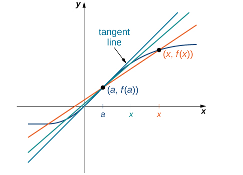
This process demonstrates how the slope of the tangent line at a particular point [latex]a[/latex] is the limit of the slopes of the secant lines, providing the derivative of the function at [latex]a[/latex], denoted by [latex]f′(a)[/latex].
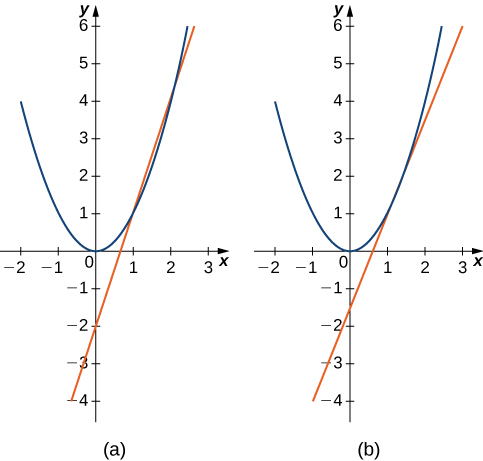
Estimate the slope of the tangent line (rate of change) to [latex]f(x)=x^2[/latex] at [latex]x=1[/latex] by finding slopes of secant lines through [latex](1,1)[/latex] and each of the following points on the graph of [latex]f(x)=x^2[/latex].
- [latex](2,4)[/latex]
- [latex]\left(\frac{3}{2},\frac{9}{4}\right)[/latex]