- Identify the line that just touches a curve at one point by looking at how nearby lines approach it
- Describe how integration can be used to calculate the area under a curve
The Tangent Problem and Differential Calculus
Variable Rate of Change
Calculus emerges from two fundamental problems: (1) the tangent problem, or how to determine the slope of a line tangent to a curve at a point; and (2) the area problem, or how to determine the area under a curve. The concept of the rate of change is pivotal in addressing these challenges.
A clear starting point for understanding the rate of change is through linear functions, which exhibit a constant rate throughout. Consider the functions [latex]f(x)=-2x-3, \, g(x)=\frac{x}{2}+1[/latex], and [latex]h(x)=2[/latex] represented graphically by straight lines. The slopes of these functions, constant across their graphs, illustrate how changes with .
For [latex]f(x)=-2x-3[/latex], a decrease in [latex]x[/latex] by one unit leads to a two-unit drop in [latex]y[/latex], illustrating a slope of [latex](−2)[/latex]. Conversely, the slope of [latex]\frac{1}{2}[/latex] in the function [latex]g(x)[/latex] gently rises, increasing [latex]y[/latex] by half a unit for each increment in [latex]x[/latex]. The function [latex]h(x)=2[/latex] has a slope of zero, indicating that the values of the function remain constant.
These linear function examples, with their constant rates of change, set the groundwork for examining functions with variable rates of change, a central inquiry of calculus.
Compare the graphs of the three linear functions with the graph of [latex]k(x)=x^2[/latex] (Figure 2).
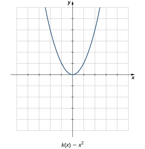
The graph of [latex]k(x)=x^2[/latex] starts from the left by decreasing rapidly, then begins to decrease more slowly and level off, and then finally begins to increase—slowly at first, followed by an increasing rate of increase as it moves toward the right. Unlike a linear function, no single number represents the rate of change for this function.
These leads to the question: How do we measure the rate of change of a nonlinear function?